Protein_Contact_Network_Explorer-PCNE-
Protein Contact Network Explorer (PCNE)
![]()
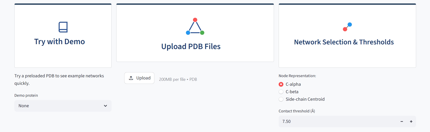
PCNE (Protein Contact Network Explorer) is an interactive web-based tool for constructing, visualising, and analysing Protein Contact Networks derived from PDB structure files. It supports three node representation modes which are Cα, Cβ, and Side-chain Centroid and computes key topological metrics including node degree, clustering coefficient, and betweenness centrality with z-score based classification of residues into Peripheral, Structural Hub, Bottleneck, and Global Critical Hub categories. Community detection is implemented via the Leiden algorithm with per-community DSSP secondary structure composition reporting. Visualisations include an interactive 2D contact network, adjacency and distance heatmaps, and an embedded 3D NGL Viewer with a toggle between betweenness centrality gradient and community membership colouring. Networks can be exported in SIF format for downstream Cytoscape integration.
Live Application: https://lactdr5rfibhg9m5tmamwg.streamlit.app/
Table of Contents
Screenshots
 |
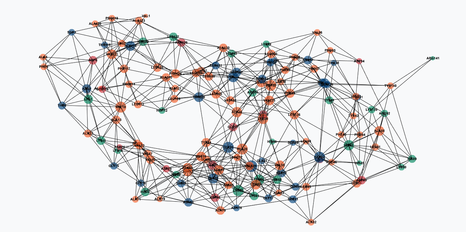 |
| Input panel with node representation selector | Full 2D contact network |
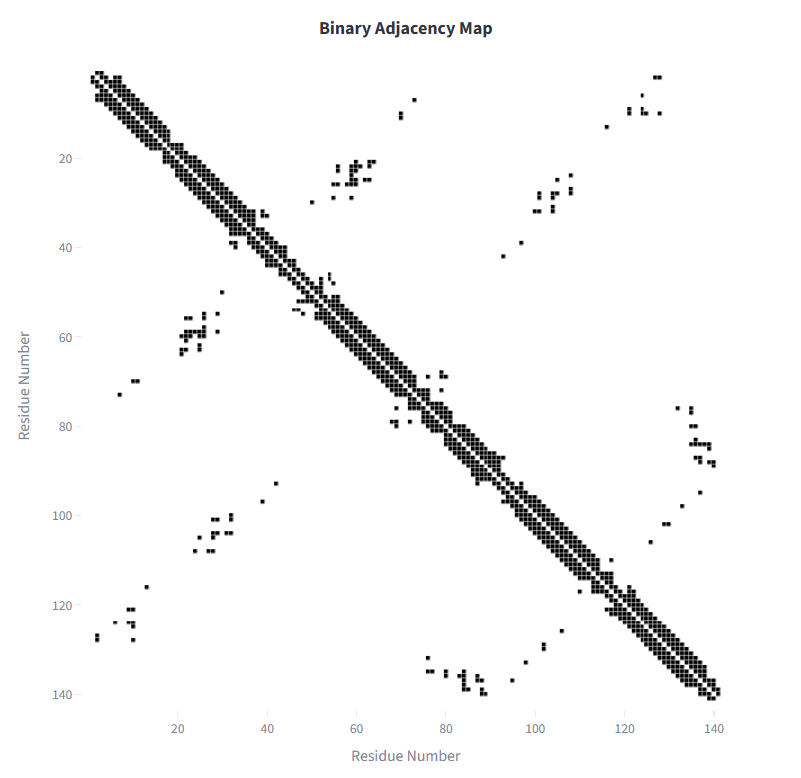 |
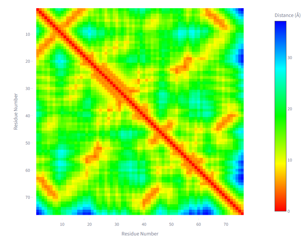 |
| Binary adjacency map | Pairwise distance heatmap |
 |
 |
| Degree vs betweenness centrality classification | Leiden community detection with DSSP composition |
 |
 |
| 3D structure coloured by betweenness centrality | 3D structure coloured by community membership |
Features
- Network Construction — accepts PDB files from X-ray crystallography and NMR ensembles with three node representation modes: Cα, Cβ, and Side-chain Centroid, each with calibrated default cutoffs.
- Topological Metrics — computes node degree, local clustering coefficient, Wasserman-Faust normalised closeness centrality, and betweenness centrality with z-score based classification into four functional residue categories.
- Community Detection — Leiden algorithm with modularity Q reporting and per-community DSSP secondary structure composition breakdown
- 3D Visualisation — embedded NGL Viewer with toggle between betweenness centrality gradient colouring and Leiden community membership colouring
- Interactive 2D Network — multiple filtering modes including hub view, hydrophobic core, closeness centrality, and betweenness views with biochemical residue type colouring
- Export — SIF format export for Cytoscape integration and matrix downloads
Methodology
Network Construction
Each residue is represented as a node. Edges are defined by Euclidean distance between residue coordinate representations. A binary adjacency matrix is constructed using a user-defined cutoff rc:
\[d(i,j) = \sqrt{(x_i - x_j)^2 + (y_i - y_j)^2 + (z_i - z_j)^2}\] \[A(i,j) = \begin{cases} 1 & d(i,j) \leq r_c \\ 0 & d(i,j) > r_c \end{cases}\]PCNE supports three node representation modes. The figure below illustrates how the measured inter-residue distance differs across representations:
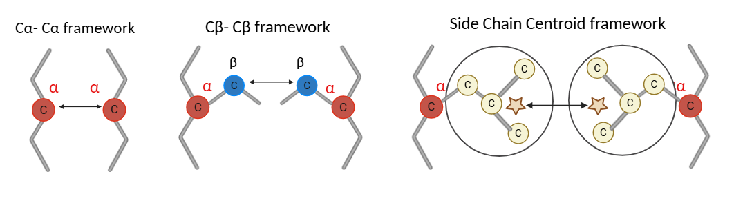
Figure 1: Node representation modes. Cα uses the alpha carbon, Cβ uses the beta carbon, and Side-chain Centroid uses the mean position of all non-hydrogen side-chain heavy atoms. Distance is measured between the respective reference points of neighbouring residues.
For the Side-chain Centroid mode, the centroid position is computed as:
\[\vec{r}_i^{\,SC} = \frac{1}{N_i} \sum_{k=1}^{N_i} \vec{r}_{i,k}\]where $N_i$ is the number of side-chain heavy atoms and $\vec{r}_{i,k}$ is the coordinate vector of the k-th heavy atom. Glycine, which has no side-chain heavy atoms, falls back to its Cα position.
Topological Metrics
PCNE computes four graph-theoretic metrics per residue: degree (number of contacts), local clustering coefficient (local cohesiveness), Wasserman-Faust normalised closeness centrality (global reachability), and betweenness centrality (information flow bottleneck score).
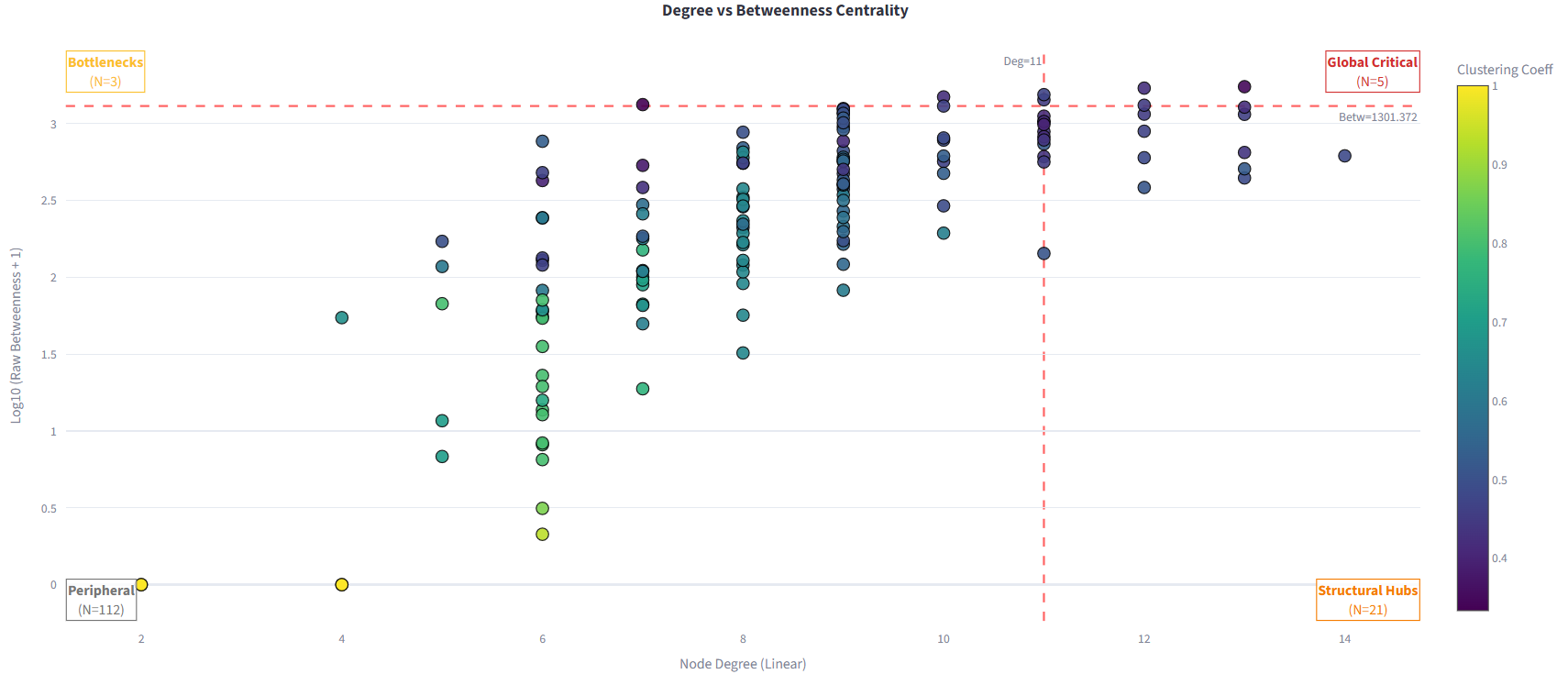
\[C_{between}(i) = \sum_{s \neq i \neq t} \frac{\sigma_{st}(i)}{\sigma_{st}}\]Residues are classified into four functional categories using z-score thresholds applied jointly to degree and betweenness distributions:
| Category | Degree | Betweenness |
|---|---|---|
| Global Critical Hub | High | High |
| Structural Hub | High | Low |
| Bottleneck | Low | High |
| Peripheral | Low | Low |
Figure 2: Residue classification by degree and betweenness centrality into four functional roles.
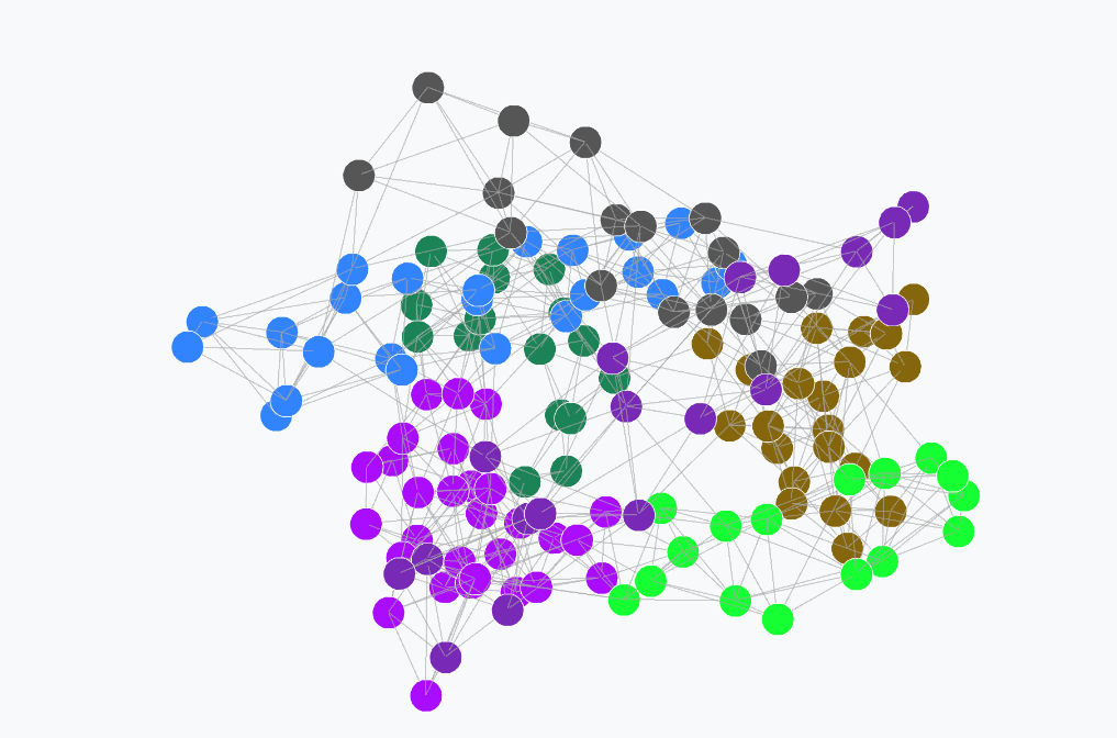
Community Detection
Community structure is identified using the Leiden algorithm optimising modularity Q. Partition quality is reported as modularity Q directly within the interface.
\[Q = \frac{1}{2m} \sum_{i,j} \left[ A_{ij} - \frac{k_i k_j}{2m} \right] \delta(c_i, c_j)\]Each community’s biological relevance is assessed through per-community DSSP secondary structure composition, reporting the fraction of helix (H), strand (E), and coil (C) residues per cluster.
Figure 3: Leiden community detection with per-community secondary structure composition bars.
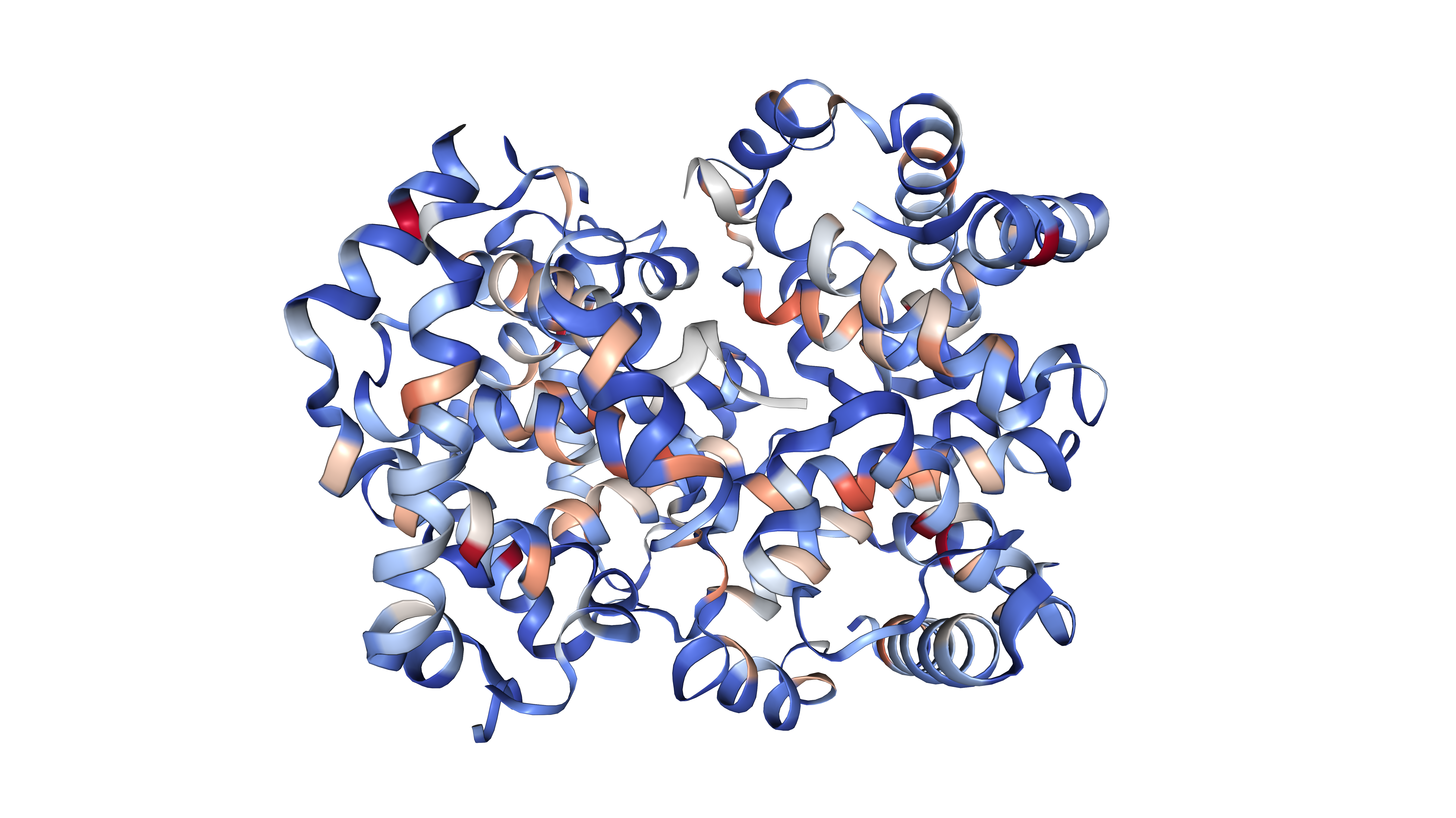
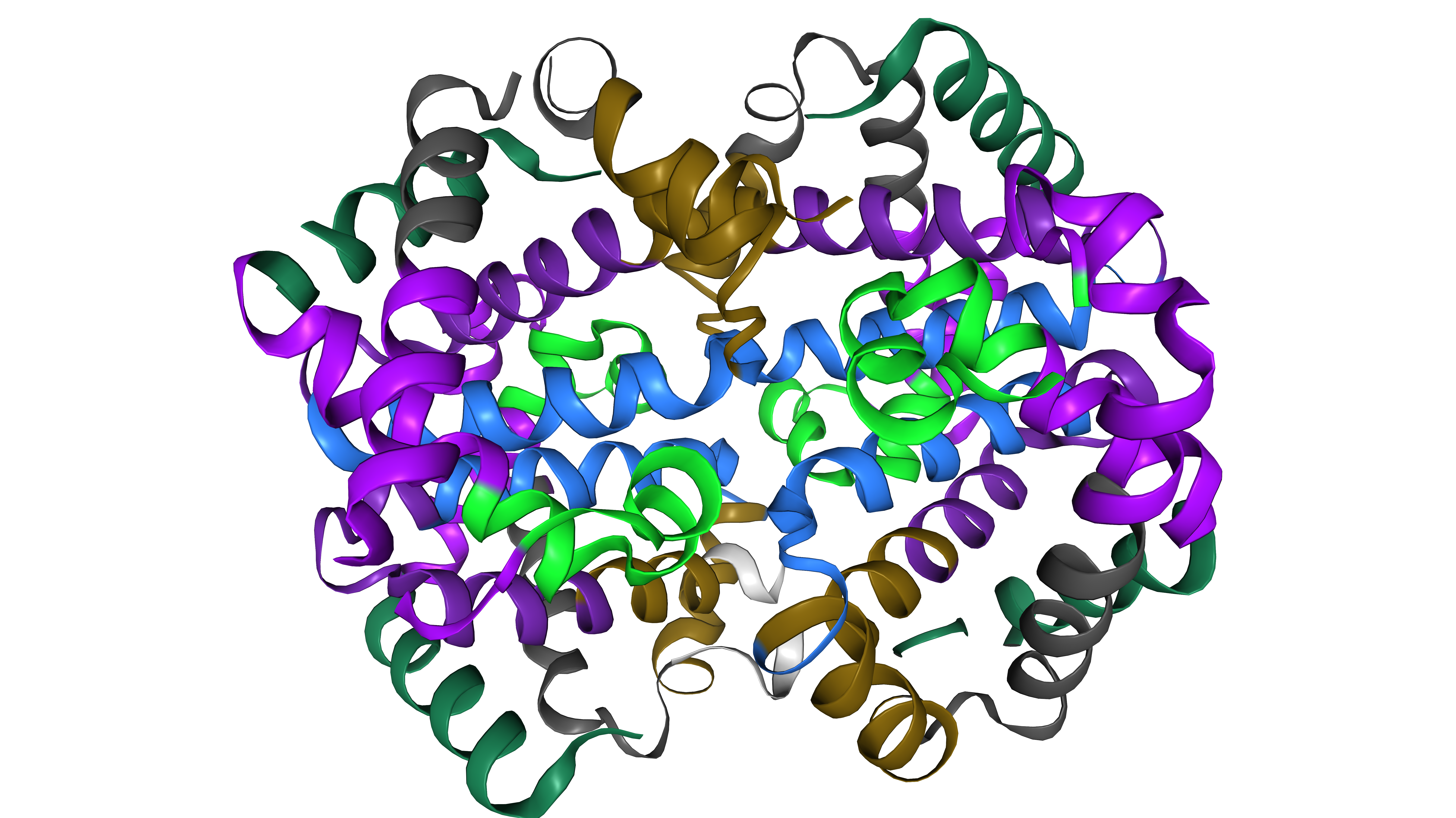
3D Visualisation
The embedded NGL Viewer renders the protein backbone in cartoon representation coloured either by log-normalised betweenness centrality using a coolwarm gradient, or by Leiden community membership using a consistent qualitative colour palette.
\[c_i^{\text{norm}} = \frac{\log(1 + BC_i) - \log(1 + BC_{\min})} {\log(1 + BC_{\max}) - \log(1 + BC_{\min})}\] |
|
| Betweenness centrality gradient | Leiden community membership |
Figure 4: 3D structure viewer with toggle between centrality and community colouring.
Installation
git clone https://github.com/akhuuu2303/Protein_Contact_Network_Explorer-PCNE-
cd Protein_Contact_Network_Explorer-PCNE-
pip install -r requirements.txt
streamlit run app.py
Requirements
streamlitbiopythonnetworkxnumpyscipypandasplotlyleidenalgigraphscikit-learn-
pillow
Usage
- Upload a PDB file or select a demo protein from the provided list
- Select node representation (Cα, Cβ, or Side-chain Centroid) and set the contact distance threshold
- Explore the network views, community detection, 3D structure viewer, and export results in SIF format for Cytoscape
Citation
If you use PCNE in your research, please cite:
@article{ganapathy2026pcne,
  title   = {Protein Contact Network Explorer: Topological Analysis
             of Protein Structures},
  author  = {Ganapathy, Akhurath and Krishnan, Sanjana V
             and Emerson, Arnold},
  journal = {Frontiers in Bioinformatics},
  year    = {2026}
}
Acknowledgements
The authors thank Vellore Institute of Technology (VIT), Vellore, for providing the infrastructure to support this work.